Mathematica Cheat Sheet

              f[x_,y_] := 1-(x-4)^2-(y-3)^2 or equivalently,

              g = 1-(x-4)^2-(y-3)^2

              Grad[f[x,y],{x,y}] or equivalently,

              Grad[g,{x,y}]

              sys = { 2x + y == 10, y/x == 2 }

              Solve[ sys, {x,y} ]

x*y /. { x -> 2.5, y -> 5}

Mathematica Tutorial

Essential Commands for Economics

Sérgio O. Parreiras

Economics Department, UNC at Chapel Hill

Computer Algebra Systems (CAS)

CAS are extremely useful for economic modelling.
There are several CAS in the market:
1. Mathematica
2. Maple (too expensive for individuals)
3. SymPy (free and open source!)
Why Mathematica?
1. UNC has license (no direct cost to you)
2. Mathematica is more user-friendly than Sage

Navigate Workbook Cells

Everything you type goes into cells: brackets on the right delimit them
Press shift+enter to execute and create a new cell.
Press enter alone to add a line within the current cell.
Use arrow keys to move between cells.
Put one command per cell for easier debugging.

Mathematica notebook window; the brackets running down the right edge delimit each cell

Define Functions

f(x) = -\exp(-\rho \cdot x)

becomes...

f[x_] := -Exp[-ρ*x]

Spot four differences:

Use square brackets for function arguments, not parentheses.
Built-in functions start with a capital letter.
Use := for definitions.
Use underscore only when defining, not when evaluating. Type f[x] then shift+enter.

Define Multi-Variable Functions

U(x,y) = 2 \cdot \ln(x) + 3 \cdot \ln(y)$$ $$V(x,y) = x^2 \cdot y^3

becomes...

U[x_, y_] := 2*Log[x] + 3*Log[y] V[x_, y_] := x^2 * y^3

* = multiplication ^ = exponentiation

Verify Your Definitions

Definitions with := produce no output. To verify, call the function:

h[x_] := x^2 <shift+enter> (no output) h[x] <shift+enter> Out= $x^2$

Tip: You can use = instead of := in most cases.

Lists (vectors)

Extract parts of a list

Write lists/vectors using curly braces: $\left(\frac{1}{3}, \frac{2}{3}, \frac{6}{9}\right) \to$ {1/3, 2/3, 6/9}

Extract elements with double brackets:

L[[k]] $\to$ $k$-th element
L[[i;;j]] $\to$ elements $i$ through $j$

Example: L = {a, 1, z, 9, 4}

L[[1]] $\to$ a L[[3]] $\to$ z
L[[2;;4]] $\to$ {1, z, 9}

Lists (vectors)

Compute Inner Products

Use a period . for dot products (element-wise multiply, then sum):

\left(\frac{1}{3}, \frac{2}{3}\right) \cdot (\ln(c_1), \ln(c_2)) = \frac{1}{3}\ln(c_1) + \frac{2}{3}\ln(c_2)

becomes...

{1/3, 2/3} . {Log[c1], Log[c2]} Out: $\frac{1}{3}\text{Log}[c_1] + \frac{2}{3}\text{Log}[c_2]$

Lists (vectors)

Apply Functions to Lists (Vectorization)

Functions automatically apply to each element of a list:

u[x_] := Sqrt[x] L = {1, 25, 9, 4, 16} u[L] $\to$ {1, 5, 3, 2, 4}

Write Equations and Systems

Use double equals == for equations (single = is for assignment).

Systems of equations are just lists of equations:

{x + y == 10, x - y == 2}

Key insight: If equations are equal to a constant—no need to expand!

FOC = Grad[f[x, y], {x, y}] == 0

is equivalent to

FOC = {D[f[x, y], x] == 0, D[f[x, y], y] == 0}

Compute Derivatives with D

Use D[f[x], x] for derivatives:

D[f[x], x]	first derivative
D[f[x, y], x]	partial w.r.t. $x$
D[f[x, y], x, y]	cross partial $\partial^2/\partial x \partial y$
D[f[x], x, x]	second derivative

Example: Arrow-Pratt risk aversion

rho = -D[f[x], x, x] / D[f[x], x]

Compute the Gradient

Use Grad to get all partial derivatives at once:

Grad[f[x, y, z], {x, y, z}]

returns:

\left\{\frac{\partial f}{\partial x}, \frac{\partial f}{\partial y}, \frac{\partial f}{\partial z}\right\}

Key application: First-order conditions (FOC)

Grad[f[x, y], {x, y}] == 0

Solve Systems of Equations

Basic syntax:

Solve[{eq1, eq2, ...}, {x, y, ...}]

Example: Equilibrium (both FOCs = 0)

Solve[{10 - 2x - y == 0, 8 - x - 2y == 0}, {x, y}]

Shortcut: Solve accepts a list equal to zero directly!

FOC = Grad[u[x, y], {x, y}] Solve[FOC == 0, {x, y}]

Solve vs Reduce

Solve: Simple syntax, general solutions only

Solve[{x + y == 10, x*y == 21}, {x, y}]

Reduce: Handles assumptions and special cases

Reduce[{x + y == m, x > 0, y > 0}, {x, y}, Reals]

Tip: Use Solve for most economics problems. Use Reduce when you need parameter restrictions or complete case analysis.

Plot Curves with ContourPlot

Plot implicit equations without solving:

ContourPlot[x^2 + y^2 == 10, {x, -5, 5}, {y, -5, 5}]

Plot multiple curves using lists of equations

ContourPlot[{x+y == 10, Sqrt[x]+Sqrt[y] == 3}, {x, 0, 10}, {y, 0, 10}]

(Budget line and indifference curve together)

Plot Regions with RegionPlot

Shade regions satisfying inequalities:

RegionPlot[x + y <= 10, {x, 0, 10}, {y, 0, 10}]

Combine conditions:

&& = "and" (intersection)
|| = "or" (union)

RegionPlot[x+y <= 10 && x >= 0 && y >= 0, {x, 0, 10}, {y, 0, 10}]

Useful Commands: Simplify, N, Substitution

Simplify[x^2 + 2x + 1]	$\to (x+1)^2$
N[1/3]	$\to 0.333333$
x^2*y /. {x -> 3, y -> 7}	$\to 63$

Substitution syntax: Type -> for $\to$

expr /. {x -> value}

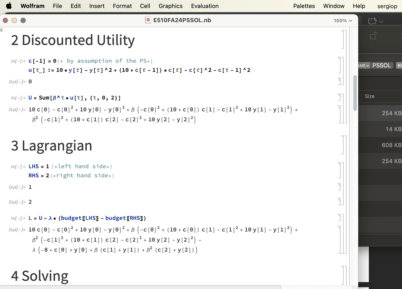
Create Indexed Variables with Table

For dynamic models, use brackets for indexing: $c_t \to$ c[t]

Generate sequences:

Table[c[t], {t, 0, 2}] $\to$ {c[0], c[1], c[2]}

Table[p[t], {t, 0, 2}].Table[c[t], {t, 0, 2}] $\to \sum_t p[t]c[t]$

Combine and sum lists:

Join[{a, b}, {c, d}] $\to$ {a, b, c, d}

Total[{a, b, c}] $\to a + b + c$

Get Help

Read this tutorial first!
Wolfram Documentation: Help $\to$ Wolfram Documentation $\to$ search command. Focus on Basic Examples.
Debug systematically:
- Put Exit[] in first cell to clear memory
- One command per cell
- Re-run cells in order with shift+enter
Still stuck after 5 min? Send me your .nb file (not screenshots).

Practice

Cournot Duopoly

Define profit functions: $u_1(q_1, q_2) = (3 - q_1 - q_2)q_1$ and $u_2(q_1, q_2) = (2 - q_1 - q_2)q_2$

Click a card to reveal the answer.

Define functions

Compute a gradient (list of all partial derivatives)

Write and solve a system of equations

Apply substitution (replacement) rules

Mathematica Tutorial

Essential Commands for Economics

Computer Algebra Systems (CAS)

Navigate Workbook Cells

Define Functions

Define Multi-Variable Functions

Verify Your Definitions

Lists (vectors)

Lists (vectors)

Lists (vectors)

Write Equations and Systems

Compute Derivatives with D

Compute the Gradient

Solve Systems of Equations

Solve vs Reduce

Plot Curves with ContourPlot

Plot Regions with RegionPlot

Useful Commands: Simplify, N, Substitution

Create Indexed Variables with Table

Get Help

Practice