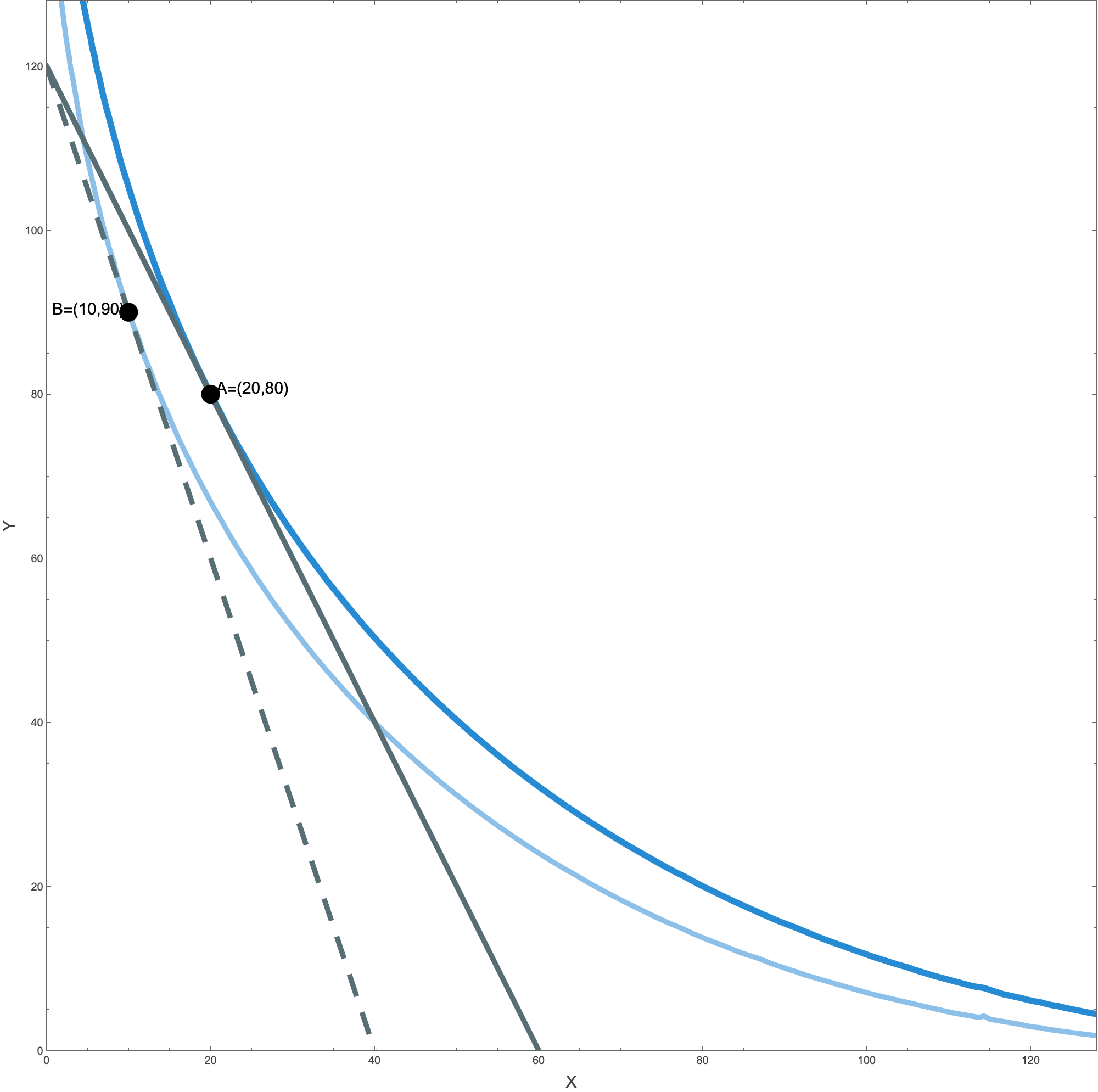
Budget lines before ($2x+y=120$, solid) and after ($3x+y=120$, dashed) the price change, with the indifference curves through the initial basket $A=(20,80)$ and the final basket $B=(10,90)$.
Individuals use as reference points:
| Economist.com offers | Price | |
|---|---|---|
| Option 1 | Web subscription | $59 |
| Option 2 | Print subscription | $125 |
| Option 3 | Print + web subscription | $125 |
Option 2 is the decoy: it costs the same as Option 3 and gives strictly less, so nobody should take it. Yet its presence makes Option 3 look like a bargain and pulls choices away from Option 1.
This model is a simplified version of Köszegi & Rabin (2006).
Let $u$ be either a utility for wealth or a gain-loss utility function. The point zero is either the initial wealth or the reference point, and we assume $u(0)=0$.
The loss-gain utility is a component of the overall utility. Its utility/disutility depends on how the consumption-utility of a good differs from the consumption-utility of its reference level.
A loss-gain utility $\mu$ as defined above displays loss aversion if and only if $L\gt G\gt 0$.
Kahneman, Knetsch & Thaler (1990) ran markets in an economics class at Cornell. Half the students, chosen at random, received an object; the other half could buy one. Since the objects were assigned at random, half of those who value them most start without one, so standard theory predicts that half of the 22 objects change hands.
| Market | Predicted trades | Observed trades |
|---|---|---|
| Induced-value tokens | supply meets demand | within one trade |
| Coffee mugs ($6.00) | 11 | 4, 1, 2, 2 |
| Ballpoint pens ($3.98) | 11 | 4 or 5 |
The median mug owner would not sell for less than $5.25, while the median buyer would not pay more than $2.25–$2.75. Median selling prices were about twice median buying prices.
A token is worth whatever the experimenter says it is worth; a mug is worth whatever its owner decides. The endowment effect shows up for the mugs and pens, not for the tokens.
Seventy-seven students at Simon Fraser University were randomly split into three groups and asked, at each price from $0.25 to $9.25, what they would do.
| Group | Decision at each price | Median price |
|---|---|---|
| Sellers | own a mug: sell it or keep it | $7.12 |
| Choosers | no mug: take a mug or the money | $3.12 |
| Buyers | no mug: buy one or keep the money | $2.87 |
Sellers and Choosers face the same choice—leave with the mug or with the money—yet Choosers price the mug like Buyers. The low volume of trade comes from owners' reluctance to part with the mug, not from buyers' reluctance to part with cash.
Owning does not make the object more attractive: students given a pen did not rate pens as more attractive than the others did, yet 56% of them kept the pen over two chocolate bars, against 24% of those not given one.
Let good $X$ be a mug, $x\in\set{0,1}$, and good $Y$ be money, with $u(y)=y$. Write $m=u(1)-u(0)\gt 0$ for the consumption utility of the mug.
Therefore $$\frac{\mathrm{WTA}}{\mathrm{WTP}}=\paren{\frac{1+L}{1+G}}^2\gt 1\iff L\gt G.$$
With the $\mu$ of the numerical example ($L=1$, $G=\tfrac12$), $\mathrm{WTA}/\mathrm{WTP}=\paren{2/\tfrac32}^2=\tfrac{16}{9}\approx 1.8$—close to the factor of about 2 in the mug markets. Without loss aversion ($L=G$) the gap vanishes: $\mathrm{WTA}=\mathrm{WTP}=m$. A Chooser gains either the mug or the money, so is indifferent at $p=m$, between the two—the same order as $\$2.87\lt\$3.12\lt\$7.12$.
Capuchins who had learned to trade tokens for food chose between two experimenters. Each experimenter first showed some apple pieces, then took a token and gave apple pieces—sometimes more, sometimes fewer than shown. Each cell below reads pieces shown → pieces given.
| Experiment | E1 | E2 | E1 chosen |
|---|---|---|---|
| 2. Gamble | 1 → 1 or 2 | 2 → 1 or 2 | 71% |
| 3. Sure thing | 1 → 1 | 2 → 1 | 79% |
Within each experiment the two experimenters deliver the same payoffs; only the display differs. Standard theory gives no reason to favor either one.
The displayed apple sets what the monkey expects—the third kind of reference point above—and getting less than that is coded as a loss. In the mug markets the reference is what one owns; here it is what one was shown.
The reference basket $r=(\bar x,\bar y)$ splits the good space into four regions. Click a region to reveal the reference-dependent consumer's $\mathrm{MRS}$ there.
A consumer looks for the optimal basket $(x,y)$ on the budget line $p_X\,x+p_Y\,y=I$.
That happens in one of two ways:
Consider a traditional ($T$) consumer with utility $u_T(x,y)=\sqrt{x}+\sqrt{y}$, a consumer ($R$) with reference dependent utility, $$u_R(x,y\mid 20,80)=\sqrt{x}+\sqrt{y}+\mu(\sqrt{x}-\sqrt{20})+\mu(\sqrt{y}-\sqrt{80}),$$ where:
We assume that both consumers' incomes are $I_T=I_R=120$ and prices initially are $p_X=2$ and $p_Y=1$.
At these prices, the optimal choice for these consumers is to choose the basket $(20,80)$, which (by chance) coincides with the reference basket of the $R$ consumer.
Now suppose the price of $X$ rises to $p_X=3$ (with $p_Y=1$ and $I=120$ unchanged), so the budget line pivots about its $Y$-intercept $(0,120)$.
Budget lines before ($2x+y=120$, solid) and after ($3x+y=120$, dashed) the price change, with the indifference curves through the initial basket $A=(20,80)$ and the final basket $B=(10,90)$.
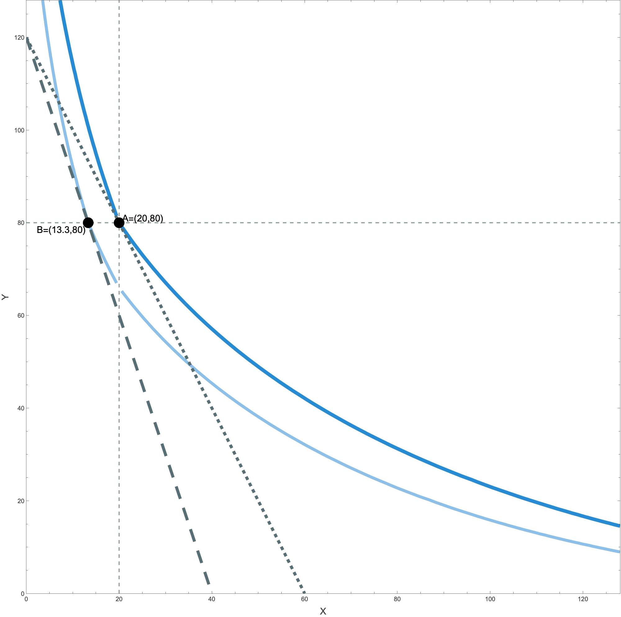
The same budget change. The indifference curves are kinked along the reference lines $x=\bar x$ and $y=\bar y$ (dotted). The consumer moves from $A=(20,80)$ to $B\approx(13.3,80)$, staying on the $y=\bar y$ kink line—$Y$ pinned at its reference level.