← back to index

Recitation 14

Loanable Funds, Savings, and Bond Pricing

Problem 2: Google's Project Decisions and Demand for Loanable Funds

The financial analysts at Google have evaluated five major projects. Each project, if it actually goes forward, will be financed by going to a bank to borrow the money. They've calculated a "break-even interest rate": If they can borrow cash to pay for the project at less than that rate, the project will likely be a success; if the rate is higher, then it's not worth it.

Project Cost Break-even Interest Rate
Project A $100 million 8%
Project B $50 million 12%
Project C $200 million 5%
Project D $25 million 4%
Project E $150 million 10%

(a) If the interest rate is 11%, which projects will Google take on? If the market interest rate is 6%, which projects will it take on?

(b) Let's turn this information into a demand curve for loanable funds. Organize this data to convert it into Google's "loanable funds demand" curve. Note: It will look just like an ordinary demand curve, only with more breaks.
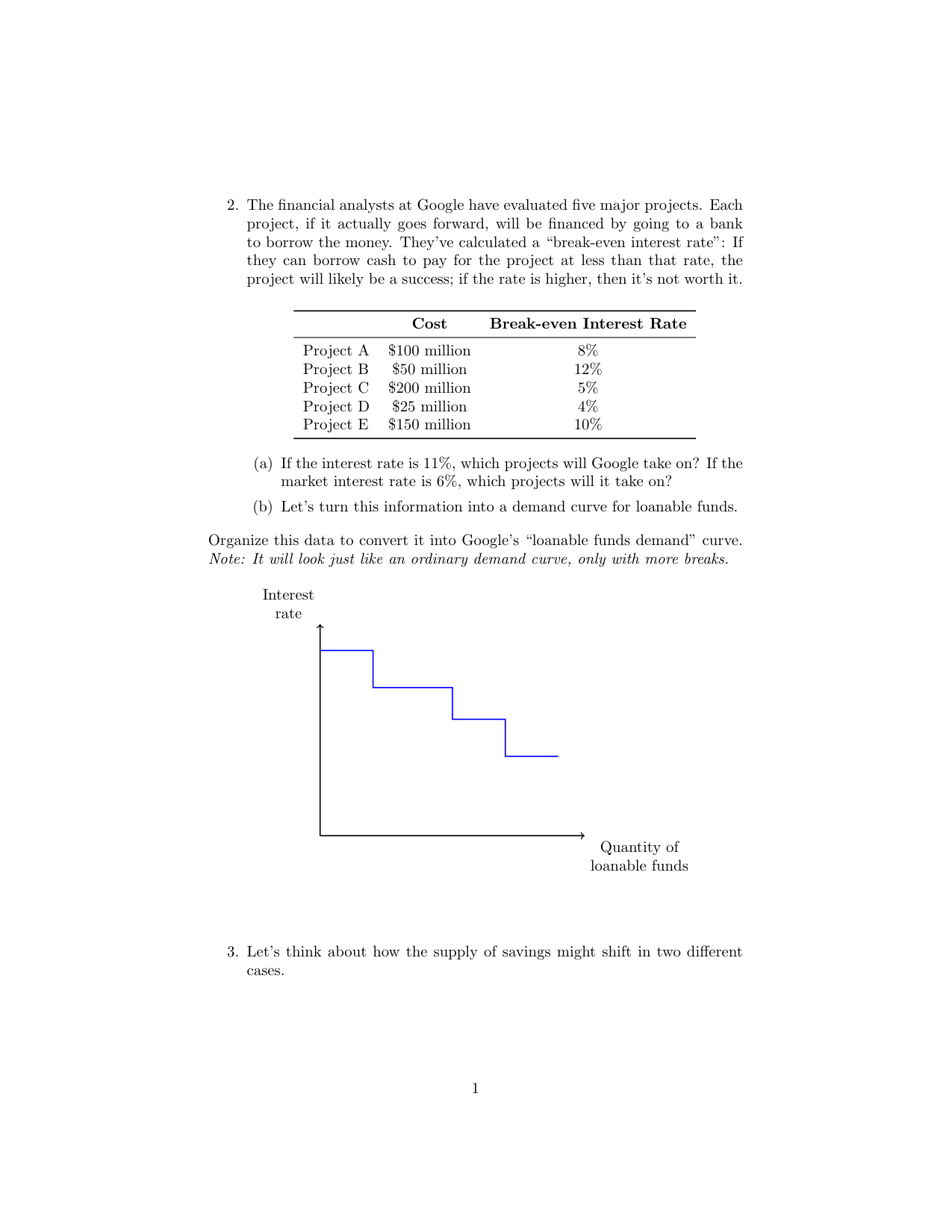
Blank demand curve template with Interest rate on y-axis and Quantity of loanable funds on x-axis
Template for demand curve (part b).

Decision rule: Take on a project only if the market interest rate is strictly less than the project's break-even rate (otherwise borrowing costs swallow the project's returns).

(a) Which projects at 11% and at 6%?

At an interest rate of 11%: Only Project B (break-even 12%) clears the bar.

  • Project B: 12% > 11% ✓ Undertake
  • Projects A, C, D, E: break-even rates (8%, 5%, 4%, 10%) are all below 11% — skip.

Answer: At 11%, Google undertakes Project B only, borrowing $50 million.

At an interest rate of 6%: All projects with break-even rates above 6% are profitable.

  • Project B (12%), Project E (10%), Project A (8%): all above 6% ✓
  • Project C (5%) and Project D (4%): below 6% — skip.

Answer: At 6%, Google undertakes Projects A, B, and E, borrowing \(100 + 50 + 150 = 300\) million, or $300 million.

(b) Demand curve for loanable funds

Rank projects from highest break-even rate (taken first) to lowest, and accumulate the borrowed amount:

Project Break-even Rate Cost Cumulative Quantity Demanded
B 12% $50M $50M
E 10% $150M $200M
A 8% $100M $300M
C 5% $200M $500M
D 4% $25M $525M

Answer: Each horizontal segment corresponds to one project; the vertical drops occur at the cumulative dollar amount where Google moves on to the next, lower-break-even project.
Problem 3a: Shifts in the Supply of Savings — Automatic Enrollment Repeal

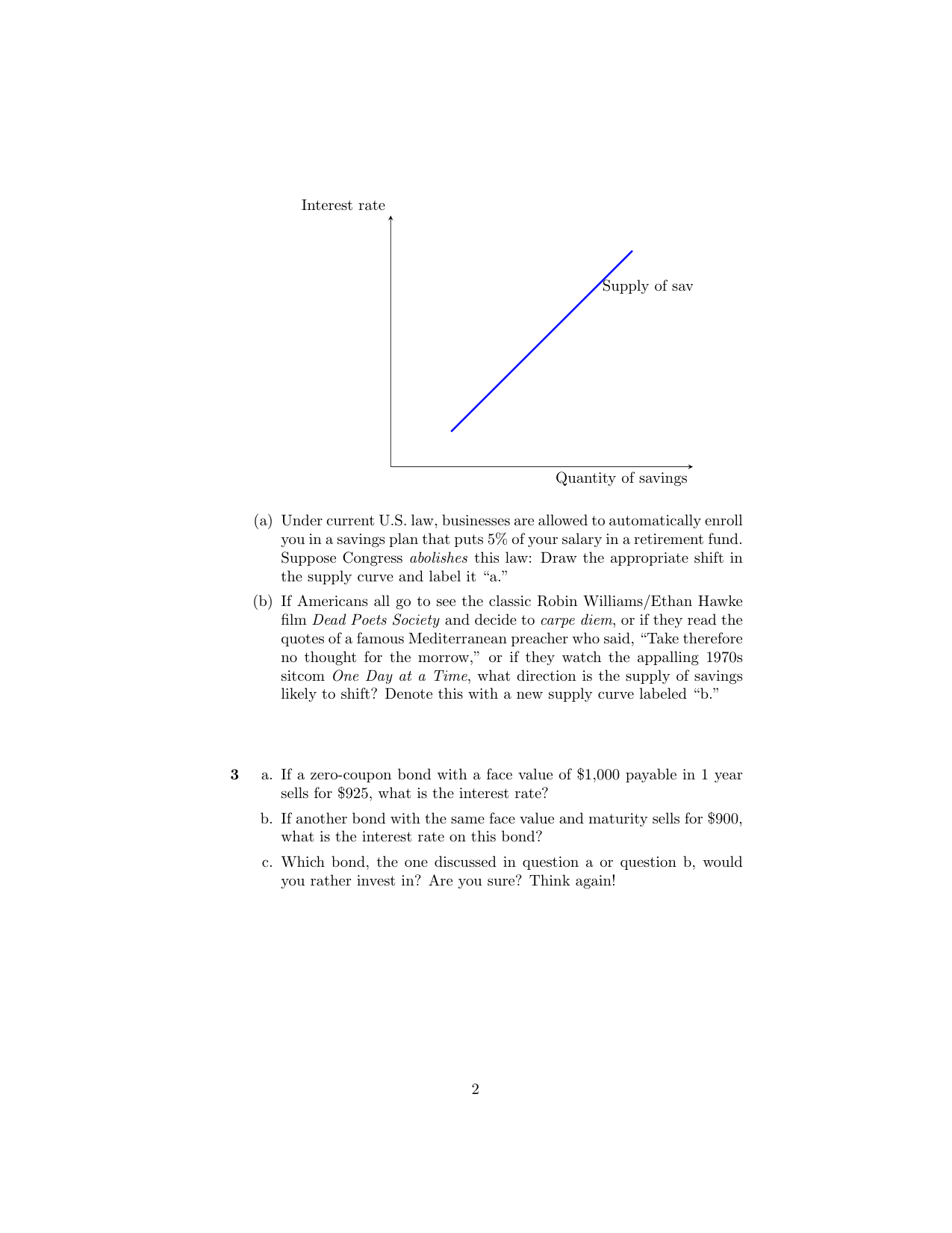
Under current U.S. law, businesses are allowed to automatically enroll you in a savings plan that puts 5% of your salary in a retirement fund. Suppose Congress abolishes this law: Draw the appropriate shift in the supply curve and label it "a."

Supply of savings curve template with Interest rate on y-axis and Quantity of savings on x-axis
Template for supply curve shifts (part 3).

Repeal of automatic enrollment in retirement plans

Auto-enrollment exploits inertia: once enrolled, most workers never opt out, so 5% of their pay flows to savings by default. If Congress abolishes the law, fewer workers would actively choose to enroll, and aggregate savings at every interest rate would fall.

Answer: The supply of savings shifts leftward (curve a). At any given interest rate, the quantity of savings is smaller.

Problem 3b: Shifts in the Supply of Savings — Cultural Messages

If Americans all go to see the classic Robin Williams/Ethan Hawke film Dead Poets Society and decide to carpe diem, or if they read the quotes of a famous Mediterranean preacher who said, "Take therefore no thought for the morrow," or if they watch the appalling 1970s sitcom One Day at a Time, what direction is the supply of savings likely to shift? Denote this with a new supply curve labeled "b."

"Carpe diem" / "take no thought for the morrow"

All three cultural messages encourage present-oriented consumption rather than future-oriented saving. If Americans collectively become more present-biased, they save less at every interest rate.

Answer: The supply of savings also shifts leftward (curve b).

Problem 3: Zero-Coupon Bond Yields

A zero-coupon bond pays the face value at maturity and nothing in between. For a bond with face value \(F\) maturing in one year at price \(P\), the implicit interest rate \(i\) satisfies:

\[ P = \frac{F}{1+i} \quad \Longleftrightarrow \quad i = \frac{F - P}{P} \]

a. If a zero-coupon bond with a face value of $1,000 payable in 1 year sells for $925, what is the interest rate?

b. If another bond with the same face value and maturity sells for $900, what is the interest rate on this bond?

c. Which bond, the one discussed in question a or question b, would you rather invest in? Are you sure? Think again!

a. Bond A: \(F = \$1,000\), \(P = \$925\)

\[ i_A = \frac{1000 - 925}{925} = \frac{75}{925} \approx 0.0811 = 8.11\% \]

Answer: The interest rate on Bond A is approximately 8.11%.

b. Bond B: \(F = \$1,000\), \(P = \$900\)

\[ i_B = \frac{1000 - 900}{900} = \frac{100}{900} \approx 0.1111 = 11.11\% \]

Answer: The interest rate on Bond B is approximately 11.11%.

c. Which bond would you rather invest in? Think again!

First instinct: Bond B looks better — a higher yield (11.11% vs. 8.11%) on the same face value and same maturity.

Think again: If two otherwise-identical bonds trade at noticeably different prices, the market is telling us something. The cheaper bond (Bond B) almost certainly carries higher default risk — the market discounts it more heavily because there is a real chance the issuer fails to pay the full $1,000 at maturity. The extra ~3 percentage points of yield is a risk premium, not a free lunch.

Answer: The "right" choice depends on your tolerance for risk.

  • If both bonds are issued by the same borrower with identical terms, Bond B is unambiguously better (same risk, higher yield) — but in practice this would be an arbitrage opportunity that markets erase quickly.
  • More realistically, Bond B is priced lower because investors view it as riskier. A risk-averse investor may rationally prefer Bond A despite the lower yield.

The lesson: Higher yields on otherwise-similar bonds usually reflect higher risk, not a market inefficiency you can exploit.