← back to index

Recitation 12

Monetary Policy & Aggregate Demand

Problem 1: Central Banking and Velocity Shocks

Bring SRAS back into the model and play the role of a central banker reacting to a rise in velocity growth. The diagram below shows the economy growing at the potential growth rate with 10% inflation.

  1. Illustrate what happens if consumers and investors become more optimistic. Clearly label the new growth rate on the x-axis with the words "High-AD real growth," and label the new inflation rate on the y-axis with the words "High-AD inflation."
  2. Once the central banker sees this rise in AD, they decide to fully reverse it with monetary policy. In the graph, illustrate what happens if they do their job "just right."
  3. If they do their job "just right," what will the inflation rate be? Provide an exact number.
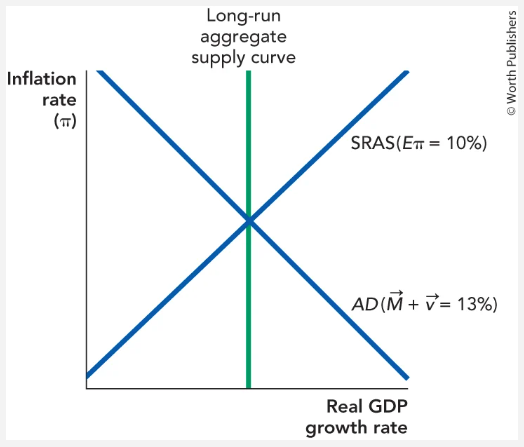
AD-AS diagram: SRAS at expected inflation 10%, AD with money growth plus velocity equal to 13%, intersecting LRAS.
Figure for Problem 1.

Part (a): AD shock from optimism

When consumers and investors become more optimistic, the AD curve shifts to the right. In the quantity-theory framework this is equivalent to an increase in velocity \( \dot{v} \), raising nominal spending growth \( \dot{M} + \dot{v} \).

  • The new AD curve intersects the SRAS to the right of the original equilibrium.
  • The intersection of the new AD with the SRAS \( (E_\pi = 10\%) \) occurs at a higher real GDP growth rate ("High-AD real growth") and a higher inflation rate ("High-AD inflation").
  • Since the SRAS is upward-sloping, both real growth and inflation rise above their initial values.

Key intuition: with expected inflation anchored at 10%, a positive demand shock moves the economy up and to the right along the SRAS, temporarily pushing real growth above potential and inflation above 10%.

Part (b): Central banker's response

To fully reverse the AD shock "just right," the central banker tightens monetary policy — reducing money growth \( \dot{M} \) by exactly enough to offset the increase in velocity \( \dot{v} \).

  • The AD curve shifts back to the left, returning to its original position: \( AD(\dot{M} + \dot{v} = 13\%) \).
  • The economy returns to the original equilibrium: real GDP growth at the potential growth rate, and inflation at 10%.
Part (c): Inflation rate if done "just right"

\[ \pi = 10\% \]

If the central banker perfectly offsets the velocity shock by reducing \( \dot{M} \) by the same amount that \( \dot{v} \) increased, nominal spending growth remains at 13%. The economy stays at the intersection of the original AD curve and the LRAS, and inflation remains exactly 10%.
Problem 2: Managing Inflation Expectations

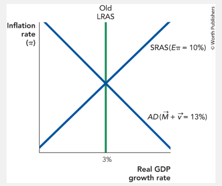
Central bankers must manage expectations. Suppose inflation is running at 10% and the central banker would like to lower inflation to 2% without reducing real growth. Assume velocity shocks are zero and the potential growth rate is 3%.

  1. What should the central banker tell the public, and at what level should the central banker set money growth?
  2. Suppose the public believes the central banker. What temptation might the central banker face? (Hint: imagine an election year and the central banker would like to see the current administration reelected.)
AD-AS diagram with Old LRAS marked, SRAS at expected inflation 10%, AD with money growth plus velocity equal to 13%, real GDP growth marked at 3%.
Figure for Problem 2.

Part (a): Lowering inflation without reducing real growth

From the quantity theory:

\[ \dot{M} + \dot{v} = \pi + g_Y \]

With \( \dot{v} = 0 \), potential growth \( g_Y^* = 3\% \), and target inflation \( \pi^* = 2\% \):

\[ \dot{M} = \pi^* + g_Y^* - \dot{v} = 2\% + 3\% - 0\% = 5\% \]

What the central banker should tell the public:

"We are committed to bringing inflation down to 2%. We will set money growth at 5% and maintain it. You should update your inflation expectations to 2%."

Mechanism: the central banker must credibly commit so the SRAS shifts down. If the public believes the announcement and lowers expected inflation to 2%, \( SRAS(E_\pi = 10\%) \) shifts down to \( SRAS(E_\pi = 2\%) \). The new equilibrium is

\[ \pi = 2\%, \quad g_Y = g_Y^* = 3\% \]

Real growth is preserved because the disinflation is costless when fully credible — the economy moves straight down along the LRAS rather than going through a costly recession.

Part (b): Time-inconsistency / temptation to inflate

Once expectations are anchored at 2%, the central banker has an incentive to deviate (time inconsistency):

  • The central banker could secretly increase money growth above 5% (e.g., back to 13%), shifting AD to the right.
  • Because expectations are now anchored at 2%, the economy moves up and to the right along the new \( SRAS(E_\pi = 2\%) \).
  • This produces a boom in real GDP growth above potential — politically attractive in an election year.
  • The cost (higher inflation) comes later, after the election, when expectations adjust upward and credibility is destroyed for future periods.

Problem 3: Federal Reserve Operations and AD

Use the model of supply and demand for bank reserves to explain how the Federal Reserve can change aggregate demand in the short run. The Federal Reserve controls the supply of bank reserves; private banks create the demand for bank reserves. After a meeting, the Fed's Open Market Committee votes to cut interest rates from 2% to 1.5%.

  1. How will they make this happen — will they increase the supply of reserves or decrease the supply?
  2. As a result of your answer to part (a), will banks usually lend more money in response, or less? Will this tend to increase the nation's money supply, lower it, or have no net effect?
  3. Will this typically increase aggregate demand or lower it?

Part (a): How the Fed cuts rates from 2% to 1.5%

To lower the federal funds rate, the Fed must increase the supply of reserves.

  • The reserve supply curve is vertical (perfectly inelastic) because the Fed is the monopoly supplier of reserves — it sets the quantity independent of the interest rate.
  • Reserve demand is downward-sloping: banks demand more reserves at lower interest rates (opportunity-cost argument).
  • To push the equilibrium rate down from 2% to 1.5%, the Fed shifts the vertical supply curve right by conducting open-market purchases (buying Treasury securities, crediting banks with new reserves).
  • The new intersection of the rightward-shifted supply with the downward-sloping demand yields the lower equilibrium FFR of 1.5%.
Part (b): Effect on bank lending and the money supply
  • When the FFR falls to 1.5%, the return on holding reserves at the Fed decreases.
  • The opportunity cost of lending falls: banks now give up less by lending out rather than holding reserves at the Fed.
  • Banks lend more — not merely because they have more reserves, but because holding reserves has become relatively less attractive.
  • Through the money multiplier, the additional lending creates new deposits, enabling further lending.
  • The net effect is an increase in the nation's money supply.
Part (c): Effect on aggregate demand

This will typically increase aggregate demand.

  • A higher money supply raises nominal spending: from the quantity theory, \( AD = \dot{M} + \dot{v} \), so an increase in \( \dot{M} \) shifts AD to the right.
  • Lower interest rates also directly stimulate investment and consumption (the interest-rate channel of monetary transmission).
  • The rightward shift of AD raises both real GDP growth (in the short run) and inflation.