Go to https://fred.stlouisfed.org/ and search for the "effective federal funds rate" (EFFR). Alter the series so the graph displays the value of the EFFR from July 3, 2000 through April 3, 2023.
- (a) How many recessions have there been over this time period? During those recessions, what happened to the EFFR? Provide an intuitive reason for why you are observing this trend/relationship.
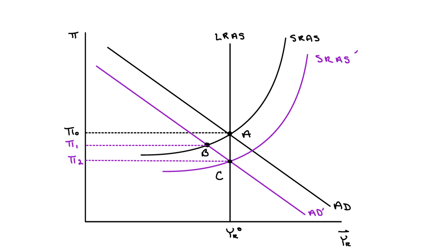
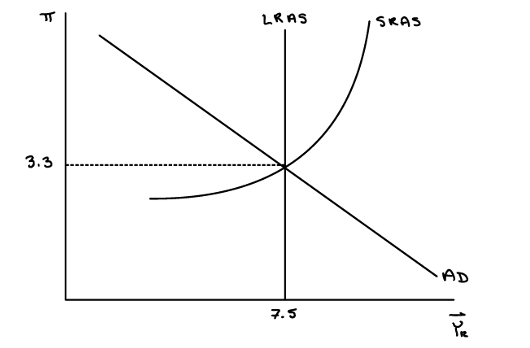
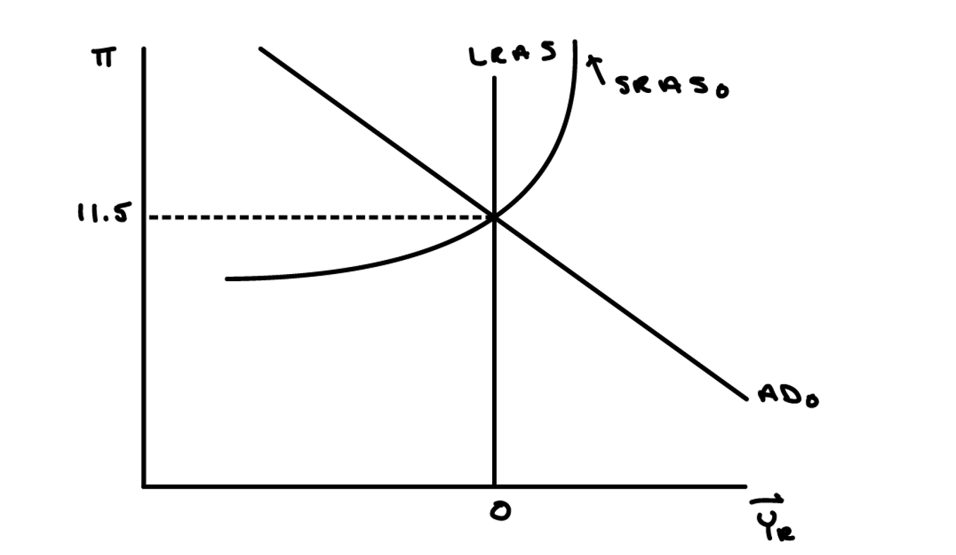
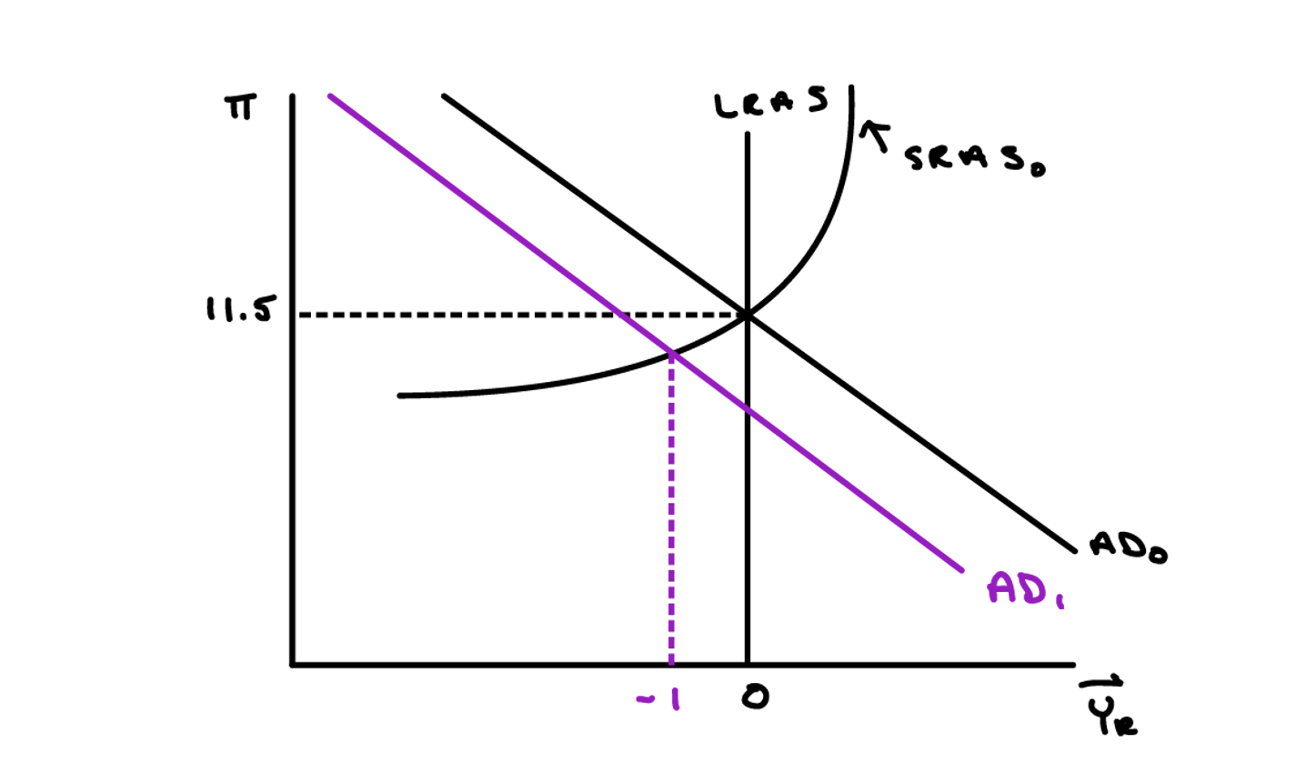
- (b) As of April 3, 2023, what is the value of the EFFR? What was the value of the EFFR one year ago? Recently, the Fed has been raising interest rates because it is concerned about inflation. Using the AD-AS model, describe the logic behind the Fed's approach. Draw a graph to support your answer.
- (c) Suppose the Fed is successful in lowering the inflation rate. Explain why over time the inflation rate may fall even further. Show this change on the graph that you drew for part (b).
Solution:
Part (a): EFFR and Recessions
There were 3 recessions during the period from July 3, 2000 through April 3, 2023:
- 2001 recession
- 2007–2009 Great Recession
- 2020 COVID recession
During each recession, the EFFR fell. This makes economic sense because:
- The Federal Reserve lowers interest rates during recessions to stimulate the economy
- Lower interest rates reduce borrowing costs for consumers and firms
- This encourages increased investment and consumption spending
- The increased spending shifts the aggregate demand (AD) curve to the right
- This policy, known as expansionary monetary policy, aims to increase real GDP growth
- If effective, it can help restore output to potential levels and reduce unemployment
Part (b): Recent Fed Rate Changes and the AD-AS Framework
EFFR values:
- As of April 3, 2023: EFFR \(\approx 4.8\%\)
- One year prior (April 3, 2022): EFFR \(\approx 0.3\%\)
Fed's Logic:
By raising interest rates, the Fed is employing contractionary monetary policy. The mechanism works as follows:
- Higher interest rates increase the cost of borrowing for households and firms
- Investment spending falls (firms find fewer projects profitable)
- Consumption spending falls (households find saving more attractive)
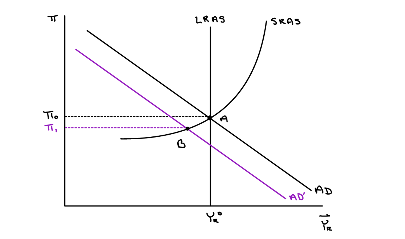
- Aggregate demand declines; the AD curve shifts leftward
- At the new equilibrium (point B), the inflation rate falls from \(\pi_0\) to \(\pi_1\) while real growth moderates
- This reduces demand-pull inflation without triggering a severe recession
Part (c): Further Inflation Decline via Expectations
Once the Fed's contractionary policy begins to lower inflation, inflation expectations begin to decline. When households and firms expect lower inflation in the future:
- Workers demand lower wage increases (expecting lower future prices)
- Firms accept lower price growth expectations
- This shifts the short-run aggregate supply (SRAS) curve downward
- At the new equilibrium (point C), inflation falls further to \(\pi_2\)
- Importantly, this downward SRAS shift occurs without further monetary tightening
- It is a self-reinforcing mechanism: lower actual inflation anchors expectations, which further reduces inflation