← back to index

Recitation 7

Monopoly

Problem 1: Monopoly Profit Maximization

Like all firms, monopolies maximize profit by producing the quantity where marginal revenue (MR) equals marginal cost (MC).

\[ MR(Q^*) = MC(Q^*) \]

Unlike perfectly competitive firms, a monopolist's profit maximization problem is the optimal trade-off between P and Q.

  • For any positive \( Q \), marginal revenue is less than the price the monopolist can charge to sell that quantity.

\[ MR(Q) = \frac{dR(Q)}{dQ} = \frac{dp(Q)Q}{dQ} = p(Q) \frac{dQ}{dQ} + \frac{dp(Q)}{dQ} Q = p(Q) + \frac{dp(Q)}{dQ} Q \]
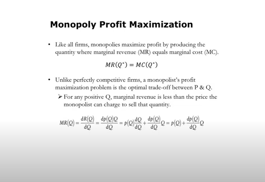
Monopoly Profit Maximization slide showing the MR=MC condition and the relationship between marginal revenue and price
Monopoly profit maximization framework.

Problem 2: MR Formula and Numerical Example

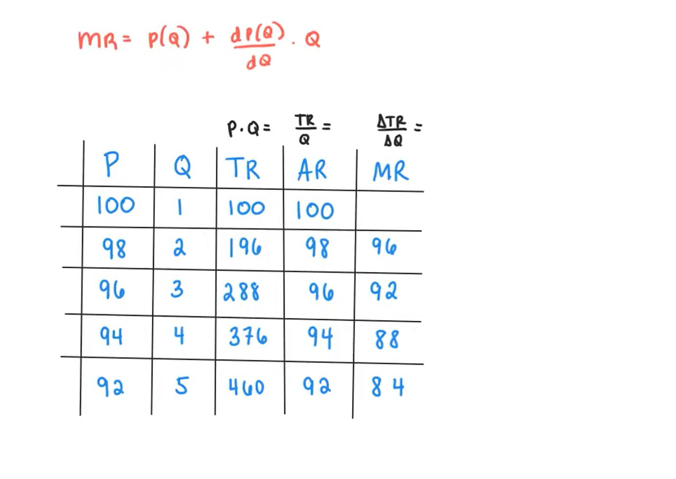
The general formula for marginal revenue:

\[ MR = p(Q) + \frac{dp(Q)}{dQ} Q \]

When the demand curve has the form \( P = a - bQ \), the marginal revenue is:

\[ MR = a - 2bQ \]

A numerical table showing the relationship between price, quantity, total revenue, average revenue, and marginal revenue:

Table showing Price, Quantity, Total Revenue, Average Revenue, and Marginal Revenue values
Numerical example: TR, AR, and MR calculations.

Problem 3: Monopoly Profit Maximization Example Problem

Given a monopolist with:

  • Demand curve: \( P = 240 - Q \)
  • Total cost: \( TC = Q^2 + 12 \)

Calculate the monopolist's profit \( \pi \).

Solution:

\( \pi = 60 \)

Explanation:

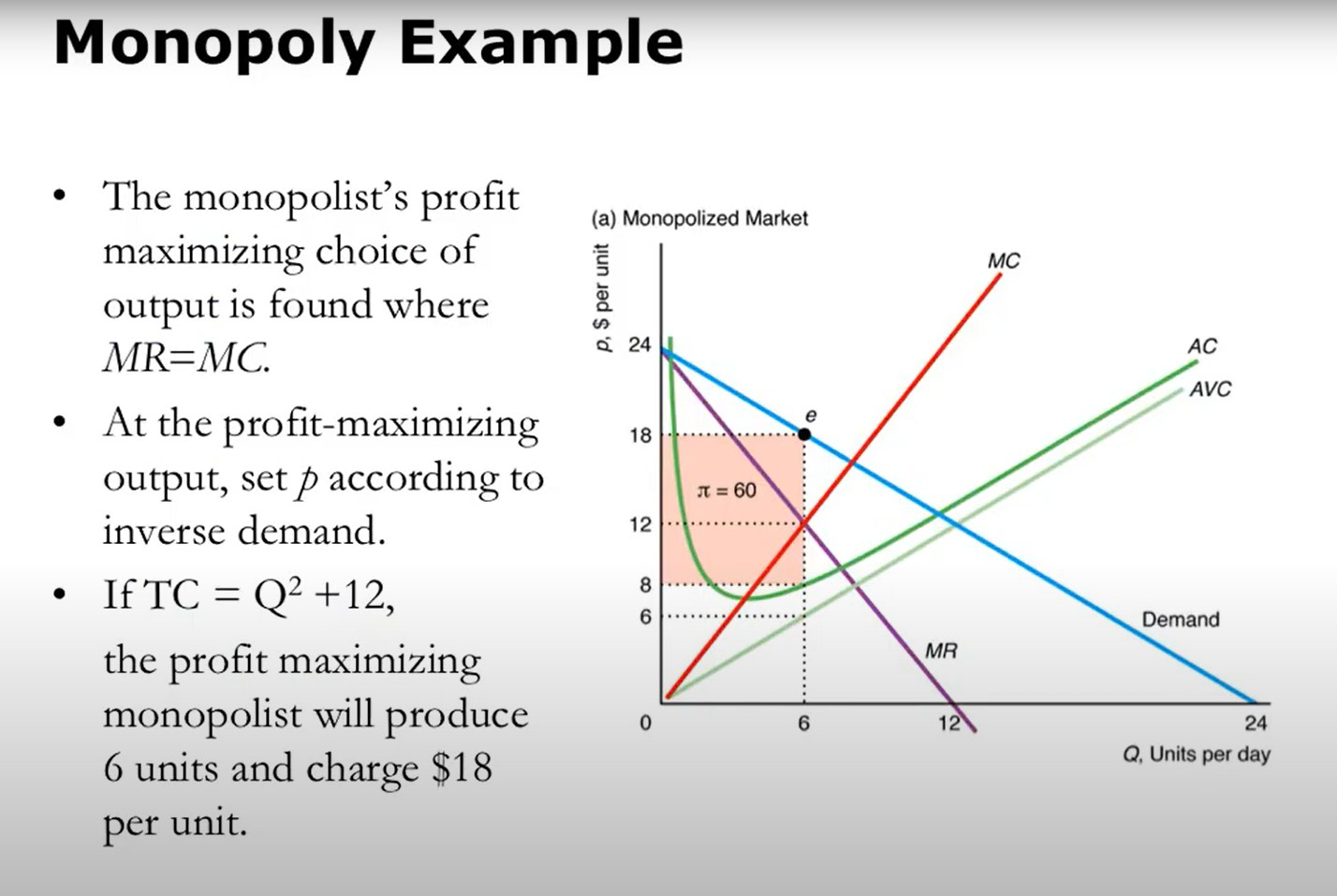
  • The monopolist's profit maximizing choice of output is found where \( MR = MC \).
  • At the profit-maximizing output, set price \( p \) according to inverse demand.
  • If \( TC = Q^2 + 12 \), the profit maximizing monopolist will produce 6 units and charge \$18 per unit.
Monopoly example diagram showing the demand curve, MR curve, MC curve, AC, and AVC curves. The profit-maximizing quantity is 6 units at price 18, with profit of 60 shown as a shaded area.
Monopoly equilibrium: MR = MC at Q = 6, P = $18, profit \( \pi \) = 60.